CGE model

Data

Closed economy

• Input-output table

• Social accounting matrix (SAM)

• SAM is a square matrix: $T= {t_{ij}}$, where $t_{ij}$ is the income from $i$ to $j$, meanwhile it is also the expenditure from $j$ to $i$
• The income must equal to expenditure: $\sum_j t_{jk} = \sum_j t_{kj}$
• For a closed economy, economic activity is divided into three categories: Consumption (C), Capital income (I) and Expenditure on production factor (Y); the income (Y) is used to consume goods and consumptions (C) and saving (S), then the saving is transformed to investment (represented by capital income (I)).

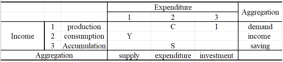
• The macro-equilibrium equation can be expressed as:
  • $Y = C + I$
  • $C + S = Y$
  • $I = S$

Open economy

• In the new table, production and consumption account is redefined as producer and residens (consumer); government is also included as an agent. In addition, the economy is open, representing by the rest of world (ROW)
• In this table, producers get income through selling the final products to residents (C) and government (G), getting profit from capital investment (I), also exporting products to ROW (E). The income is allocated into factor cost for residents (Y) and ROW (M).
• Residents’ expenditure include consumption (C), Tax (T) and saving $S_h$.
• Government’s expenditure includes consumption (G) and government saving ($S_g$)
• Income of ROW is represented by export (E) and foreign saving ($S_f$). $S_f$ is the negative value of domestic trade balance

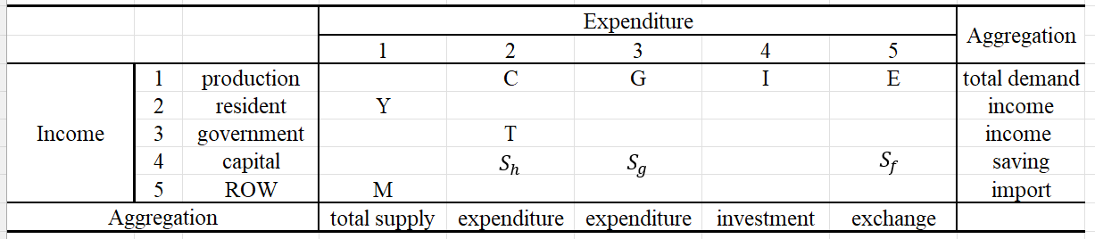
• The macro-equilibrium equation can be expressed as:
  • Gross domestic production: $Y +M = C + G + I + E$
  • Income: $C + T + S_h = Y$
  • Government Budget: $G + S_g = T$
  • Saving-investment: $I = S_g + S_h + S_f$
  • International trade balance: $E + S_f = M$
• A genral SAM is:

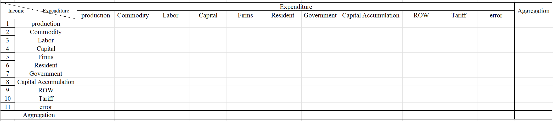
• Update SAM:
  • RAS algorithm
  • Minimizing of a constrained quadratic loss function
  • Maximum entropy tabular reconciliation
• Global trade:
  • Gravity model

Model development

Production theory

• Constant elasticity of substitution (CES)
  • For a producer, production technology is given by a CES equation under current optimal combination of factor inputs in a competitive market
    • $min \sum_i^n P_i X_i$, where $X_i$ is the production input, $P_i$ is the price
    • s.t. $ V = A[\sum_i^n a_i(\lambda_i X_i)^{\rho}]^{1/\rho}$, where $V$ is the production, $a_i$ is the share parameters. $A$ is the transformation parameter; $\lambda$ is the transformation parameter for each input
    • Specifically, neutral productivity growth is achieved by $A$, Hicks neutral production growth can only be achieved by $\lambda$
  • For the optimizaiton of producer, we set the Lagrangian equation:
    • $L = \sum_i P_i X_i + P(V-A[\sum_i a_i(\lambda_i X_i)^{\rho}]^{1/\rho})$
  • Calculate the partial differentiation for $X_i$ and $P$ and set the calculated equation equals to 0:
    • $P_i = P[\sum_i c_i X_i^{\rho}]^{\frac{1-\rho}{\rho}} c_i X_i^{\rho-1} = P V^{1-\rho} c_i X_i^{\rho-1} $
    • $V = [\sum_i c_i X_i^{\rho}]^{1/\rho}$
    • $c_i = a_i (A\lambda_i)^{\rho}$
  • Thus, we can obtain:
    • $X_i = [\frac{c_i P}{P_i}]^{\frac{1}{1-\rho}} V$
    • $V = [\sum_i c_i [\frac{c_i P}{P_i}]^{\frac{\rho}{1-\rho}} V^{\rho}]^{\frac{1}{\rho}}$
    • $P = [\sum_i c_i^{\sigma} P_i^{1-\sigma}]^{\frac{1}{1-\sigma}} = [\sum_i a_i^{\sigma}(\frac{P_i}{A \lambda_i})^{1-\sigma}]^{\frac{1}{1-\sigma}} = \frac{1}{A} [\sum_i a_i^{\sigma}(\frac{P_i}{\lambda_i})^{1-\sigma}]^{\frac{1}{1-\sigma}}$
      • Where the relationship between substitution elasticity and CES parameter is: $\sigma = \frac{1}{1-\rho}$, and $\rho = \frac{\sigma-1}{\sigma}$
  • Concequently, the factor input can be derived:
    • $X_i = (A\lambda_i)^{\sigma-1} a_i^{\sigma} (\frac{P}{P_i})^{\sigma}V$
  • If $A$ is simplified as 1 and $\lambda$ is introduced into initial share parameter:
    • $P = [\sum_i \alpha_i (\frac{P_i}{\lambda_i})^{1-\sigma}]\frac{1}{1-sigma}$
    • $X_i = \alpha_i \lambda_i^{\sigma-1}(\frac{P}{P_i})^{\sigma} V$, where $\alpha_i = a_i^{\sigma}$
    • This equation implies that the CES is a dual price system, representing the average weighted price of production inputs by productivity and input share.
    • If the price of input $i$ increases, the demand for this input will decline, and the extent of decline is determined by the substitution elasticity.
    • When the substitution elasticity equals to 0, the proportion of input demand is fixed, which is unrelated to relative price. This is the Leotief technology or fixed coefficients technology.
  • For two inputs $i$ and $j$:
    • $\frac{X_i}{X_j} = \frac{\alpha_i \lambda_i^{\sigma-1}}{\alpha_j \lambda_j^{\sigma-1}}(\frac{P_j}{P_i})^{\sigma}$
    • The substitute elasticity measures the currency value of the percentage change of the two investment ratios and the relative price percentage change
    • $\frac{\partial{\frac{X_i}{X_j}} \frac{P_i}{P_j}}{\partial{\frac{P_i}{P_j}} \frac{X_i}{X_j}}=-\sigma $
    • In the price of labor increased by 10% relative to capital, the ratio of labor demand and capital demand will decrease 10%$\sigma$
  • In most cases, we do not need the share parameter $a_i$ and $\rho$, they are defined as:
    • $a_{a,0} = (\frac{P_{i,0}}{P_0})^{\sigma}\frac{X_{i,o}}{V_0}$
    • $\alpha_i = \frac{\alpha_{i,0}}{\sum_i \alpha_{i,0}}$
    • $A = (\sum_i \alpha_{i,0})^{1/{\sigma-1}}$
• Cobb-Douglas production function
  • When the $\sigma$ is 1 and $\rho \to 0$, the production function can be written as:
    • $V = A \prod_i (\lambda_i X_i)^{\alpha_i}$, and the $\sum_i \alpha_i = 1$
    • $P = \frac{1}{A}\prod_i(\frac{P_i}{\alpha_i \lambda_i})^{\alpha_i}$
    • $X_i = \alpha_i \frac{P}{P_i}V$
    • Sometimes, we need use $PV = \sum_i P_i V_i$ to replace the dual price, making the substitute elasticity is approximate to 1.
• Leontief production function
  • When the substitute elasticity equals to 0 ($\rho \to -\infty$):
    • $V = min(\frac{\lambda_i X_i}{\alpha_i})$
    • $P = \sum_i \alpha_i(\frac{P_i}{\lambda_i})$
    • $X_i = \frac{\alpha_i}{\lambda_i}V$
• Constant-elasticity-of-transformation (CET):
  • CET is given the constraints of CET production technology, while the CES is given the CES production technology or utility function
    • max $\sum_i P_i X_i$
    • s.t. $V = (\sum_i g_i X_i^v)^{1/v}$
    • These two equations depict the producer how to distribute their goods in each market to maximize the profit
    • $X_i$ is the supply in market $i$ with a price $P_i$, and $V$ is the aggregation from all markets.
    • Where $P = (\sum_i \gamma_i P_i^{1+w})^{1/(1+w)}$, and $X_i = \gamma_i(\frac{P_i}{P})^w V$
    • And $w = \frac{1}{v-1}, w>0$, and $\gamma_i=g_i^{-w}$, $w$ is the transformed elasticity.
    • In general, $\gamma_i$ id given by: $\gamma_i = (\frac{X_{i,0}}{V_0})(\frac{P_0}{P_{i,0}})^w$
    • The difference is the definition of dual price. In CET, the substitute elasticity is positive. In supply equation, $P_i$ is in the numerator, as our expected, the increasei in price leading the increase in production.

Resident’s & consumer’s behavior

• CES utility (elasticity of commodity and income is 1)
  • General form
    • max $U = (\sum_i a_i C_i^{\rho})^{1/\rho}$
    • s.t. $\sum_i P_i C_i = Y$
    • Where $C$ is the consumption of goods and services, $P$ is the price vector, and $Y$ is the net income that can be used to consumption; $a$ is the share of consumption goods $i$
  • Given the income constraint, consumer choose the combinations of goods and services with different price, to make the utility maximization:
    • $C_i = \alpha_i’ (\frac{P}{P_i})^{\sigma}\frac{Y}{P}$
    • $P = (\sum_i \alpha_i’ P_i^{1-\sigma})^{1/(1-\sigma)}$
  • The optimization problem is:
    • $\alpha_i = a_i^{\sigma}$ and $\sigma = \frac{1}{1-\rho}>0$
      • If the $\sigma$ equals to 1, consumption shares is the constants $C_iP_i/Y$
    • All equaltion is achieved for CD utility function, with the initial utility and price index:
      • $U = \prod_i C_i^{\alpha_i}$ and $P=\prod_i(\frac{P_i}{\alpha_i})^{\alpha_i}$
      • Where $\sum_i \alpha_i$, and the constraint share should be equal to $s_i$
  • The own price elasticity is given by:
    • $\frac{\partial C_i}{\partial P_i} = -\sigma \frac{C_i}{P_i} + (\sigma-1)\alpha_i(\frac{P}{P_i})^{\sigma}\frac{C_i}{P_i} = -\sigma\frac{C_i}{P_i} + (\sigma-1)\frac{C_i}{Y} C_i$
    • $\epsilon_{ii} = \frac{\partial C_i}{\partial P_i} \frac{P_i}{C_i} = -\sigma + (\sigma-1)s_i = \sigma(s_i-1)-s_i$, where $s_i$ si the expenditure share
  • The cross-rpce elasticity is:
    • $\epsilon_{ij} = \frac{\partial C_i}{\partial P_j} \frac{P_j}{C_i} = (\sigma-1)s_j = \sigma s_j - s_j$
    • and $\frac{\partial P}{\partial P_i} = \alpha_i(\frac{P}{P_i})^{\sigma} = s_i \frac{P}{P_i}$
  • We incorporate the optimal consumption function into the CES utility function can derive indirect utility function $v(P, Y)$:
    • $v(P,Y) = \frac{Y}{P}$
  • From the indirect utility function, the Marshallian demand function can be derived:
    • $C_i(P,Y) = -\frac{\partial v \partial P_i}{\partial c \partial Y} = - \frac{-YP^{-2}(\partial P / \partial P_i)}{1/P} = - \frac{\partial P}{\partial P_i} \frac{Y}{P} = \alpha_i(\frac{P}{P_i})^{\sigma} \frac{Y}{P}$
    • given the $u, P$, the solution of minimized consumption is:
      • $min \sum_i P_i C_i$
      • $s.t. u = (\sum_i a_i C_i^{\rho})^{1/\rho}$
    • We can obtain: $E(P,u) = uP$
  • Similarly, we can calculate the compensated or Hicksian demand function:
    • $H_i(P,u)=\frac{\partial E}{\partial P_i} = \frac{\partial E}{\partial P}\frac{\partial P}{\partial P_i} = \alpha_i(\frac{P}{P_i})^{\sigma} u$
    • The Hicksian-own price elasticity is:
      • $\xi_{ii} = \sigma(s_i-1)$
    • The Hicksian-cross price elasticity is:
      • $\xi_{ij}=\sigma s_j$
• Linear expenditure system: LES utility (elasticity of commodity and income can not equal to 1)
  • developed by Richard Stone & Geary
  • Basic form:
    • $U = \prod_i (C_i-\theta_i)^{\mu_i}$, where $\sum_i \mu_i=1$
    • Where $U$ is the utility, $C$ is the consumption, $\mu, \theta$ the coefficients of consumer’s consumption
  • The optimal problem is given by:
    • max $u=\prod_i (C_i-\theta_i)^{\mu_i}$
    • s.t. $\sum_i P_i C_i = Y$, where $P$ is the consumption price, $Y$ is the net income that can be used to consume goods and services
  • The first stage of Larange multiplier is:
    • $\frac{\mu_i}{C_i - \theta_i} u = P_i \lambda$
    • $\sum_i = P_i C_i = Y$
  • The Larange multiplier $\lambda$ is the marginal contribution of income:
    • $\lambda = \frac{1}{P} = \prod_i (\frac{P_i}{\mu_i})^{-\mu_i}$
  • Thus, we can obtain:
    • $C_i = \theta_i + \frac{\mu_i}{P_i}(Y-\sum_j P_j \theta_j)$, where $1 \leq i \leq n$
    • In this formula, consumption is divided into two categories: (1) basic living expenditure $\theta$ and supernumerary consumption expenditure $\mu$, some times, $\mu$ refers to marginal consumption propensity or marginal budget share.
    • $Y^* = Y - \sum_j P_j \theta_j$, refers to the supernumerary income, measured by the income excluded basic living cost
  • From these equations, we can obtain income elasticity and price elasticity:
    • $\eta_i = \frac{\partial C_i}{\partial Y} \frac{Y}{C} = \frac{\mu_i Y}{P_iC_i} = \mu_i s_i$
    • $\epsilon_{ii} = \frac{\partial C_i}{\partial P_i}\frac{P_i}{C_i} = (-\frac{\mu_i}{P_i^2}Y^{*}-\frac{\mu_i}{P_i}\theta_i\frac{P_i}{C_i} = (-\frac{1}{P_i}(C_i-\theta_i)-\frac{\mu_i \theta_i}{P_i})\frac{P_i}{C_i} = \frac{\theta_i(1-\mu_i)}{C_i}-1$
    • $\epsilon_{ij} = \frac{\partial C_i}{\partial P_j}\frac{P_i}{C_j} = - \frac{\mu_i \theta_j P_j}{P_i C_i} = - \frac{\mu_i \theta_j P_j}{s_i Y}$
• Welfare
  • Incorporate demand function and utility function, we can calculate the indirect utility function:
    • $v(P,Y) = \prod_i (C_i-\theta_i)^{\mu_i}$, or $v(P,Y) = \prod_i (\frac{\mu_i}{P_i}Y^{*})^{\mu_i} = \frac{Y^{*}}{P}$
    • Where parameter $\mu$ have been normalized.
    • Indirect utility measures the we can obtain the maximized utility given the income and price
  • For the dual theory, we can calculate the Marshallian demand function:
    • $C_i(P,Y) = \frac{\partial v / \partial P_i}{\partial v \partial Y}$
    • where $\frac{\partial v}{\partial P_i} = \frac{1}{P} \frac{\partial Y^{*}}{\partial P_i} - \frac{Y^{*}}{P^2} \frac{\partial P}{\partial P_i} = - \frac{\theta_i}{P}-\frac{\mu_i}{P_i} \frac{Y^{*}}{P}$
    • and $\frac{\partial v}{\partial Y} = \frac{1}{P} \frac{\partial Y^*}{\partial Y} = \frac{1}{P}$, $\frac{\partial P}{\partial P_i} = \frac{\mu_i}{P_i} P$
  • The optimized problem is:
    • $min \sum_i P_i C_i$
    • s.t. $\prod_i (C_i-\theta_i)^{\mu_i} = \mu$
  • The fisrt stage condition is:
    • $\lambda \mu = \frac{P_i}{\mu_i}(C_i - \theta_i)$
    • $\prod_i (C_i-\theta_i)^{\mu_i} = \mu$
  • Consequently: (s.t. and first stage, Marshallian demand)
    • $\lambda = P$
    • $E(P,\mu) = \sum_i P_i C_i = \sum_i P_i \theta_i + \mu P$
      • where $P = \prod_i(\frac{P_i}{\mu_i})^{\mu_i}$
    • Expenditure function depicts the minimized expenditure given the utility
  • Hicksian demand function can be expressed as:
    • $H_i(P,\mu) = \frac{\partial E}{\partial P_i} = \theta_i + \mu \frac{\partial P}{\partial P_i} = \theta_i +\mu \prod_i \mu_i (\frac{P_i}{\mu_i})^{\mu_i-1} \frac{1}{\mu_i} = \theta_i+\frac{\mu_i}{P_i}\mu P$
    • Measured the changes in Hicksian welfare: Hicksian equivalent variation:
      • $EV = E(P^1, \mu^1) - E(P^0, \mu^1)$
      • $EV$ measures the compensation cost of consumer’s expenditure to achieve a new welfare. If the value is positive, there is welfare loss
      • The compensated price elasticity is:
        • $\xi_{ii} = \frac{\partial H_i}{\partial P_i} \frac{P_i}{H_i} = (\mu \frac{\mu_i}{P_i} \frac{\partial P}{\partial P_i}-\mu \frac{\mu_i}{P_i^2} P) \frac{P_i}{H_i} = \mu \frac{\mu_i}{H_i} \frac{P}{P_i} (\mu_i-1) = \mu_i(\mu_i-1)\frac{Y^{*}}{P_i H_i} = (\mu_i-1) \frac{\mu_i Y^{*}}{s_i Y}$
        • $\xi_{ij} = \frac{\partial H_i}{\partial P_j} \frac{P_j}{H_i} = (\mu \frac{\mu_i}{P_i}\frac{\mu_j}{P_j}P)\frac{P_j}{H_i} = \mu_j \frac{\mu_i Y^*}{s_i Y}$
        • And $\xi_{ij} = (\mu_j - \delta_{ij})\frac{\mu_i Y^*}{s_i Y}$, where $\delta_{ij}$ is the Kronecker product, when $i=j, \delta_{ij} = 1$, otherwise $\delta{ij} = 0$
      • We can test the Slutsky equation:
        • $\xi_{ij} = \epsilon_{ij} + s_j \eta_i$
        • The compensated demand elasticity is $\epsilon_{ij} = -\frac{\mu_i}{s_i Y}(P_j \theta_j + \delta_{ij}Y^*)$
        • The substitute elasticity is $\sigma_{ij} = \frac{\xi_{ij}}{s_j} = \frac{\mu_i Y^*}{s_i s_j Y}(\mu_j-\delta_{ij})$
        • Thus, the substitution elasticity matrix is ​​symmetric.
    • Calibration:
      • Price vector $P$
      • consumption for each goods and commodity $C$
      • Income $Y$
      • Income elasticity $\eta$
      • Marginal consumption propensity:
        • $\mu_i = \frac{\eta_i P_i C_i}{Y} = \eta_i s_i$
        • $\mu_i* = \frac{\mu_i}{\sum_i \mu_i}$ and $\eta_i^* = \frac{\mu_i^*}{s_i}$
      • When estimate the equation system, we need to set one equation is 0 or add an extra equation to achieve the full rank matrix:
        • In LES system, the Frisch equation is $\phi = - \frac{Y}{Y^*} = -\frac{Y}{Y-\sum P_j \theta_j}$
      • The new price elasticisy is:
        • $\epsilon_{ii} = \frac{\theta_i}{C_i}(1-\mu_i)-1 = \frac{P_i \theta_i}{Y} \frac{1-\mu_i}{s_i}-1 = (s_i-\frac{\mu_i Y^*}{Y})(\frac{1-s_i \eta_i}{s_i})-1 = (s_i + \frac{s_i \eta_i}{\phi})(\frac{1}{s_i}-\eta_i)-1 = 1- s_i \eta_i + \frac{s_i \eta_i}{\phi}(\frac{1}{s_i}-\eta_i)-1 = -s_i \eta_i + \frac{\eta_i}{\phi} (1-s_i \eta_i)$
        • $\epsilon_{ij} = - \frac{\mu_i \theta_j P_j}{s_i Y} = - \frac{\mu_i(P_j C_j -\mu_j Y^{*})}{s_i Y} = - \eta_i (s_j - s_j \eta_j \frac{Y^{*}}{Y}) = - \eta_i s_j (1+\frac{\eta_j}{\phi})$
        • $\theta_i = C_i - \frac{\mu_i}{P_i} Y^* = C_i - \frac{s_i \eta_i}{P_i} Y^* C_i (1+\frac{\eta_i}{\phi})$
• Extended LES: incorporate saving
  • Fluch and Howe introduce the saving decision into the consumption decision to maximize intertemporal utility:
    • $U = \prod_i (C_i-\theta_i)^{\mu_i} (\frac{S}{P^s})^{\mu_s}$, and $\sum_i \mu_i+\mu_s=1$
    • Where $U$ is the utility, $C$ is the consumption, $S$ is the saving, $P^s$ is the saving price, $\mu$ is the marginal consumption propensity and $\theta$ is the basic living consumption
    • Saving is condiered as a good, with the lowest utility 0, and the $\theta_{saving}=0$. It is a price variable rather than a quantity variable.
  • The optimized problem is:
    • max $\prod_i (C_i-\theta_i)^{\mu_i} (\frac{S}{P^s})^{\mu_s}$
    • s.t. $\sum_i P_i C_i + S = Y$
    • Where $Y$ is the income and $P$ is the price vector.
  • Demand function is:
    • $C_i = \theta_i + \frac{\mu_i}{P_i}(Y-\sum_j P_i \theta_j)$, $1 \leq i \leq n$
    • $S = \mu_s (Y-\sum_j P_i \theta_j) = Y-\sum_j P_j \theta_j$
  • The income and price elasticity is:
    • $\eta_i = \frac{\mu_i Y}{P_i C_i} = \frac{\mu_i}{s_i}$, $\eta_s = \frac{\mu_s Y}{S} = \frac{\mu_s}{s}$
    • $\epsilon_i = \frac{\theta_i(1-\mu_i)}{C_i}-1$, $\epsilon_i = -1$
    • $\epsilon_{ij} = - \frac{\mu_i \theta_j P_j}{P_i C_i} = - \frac{\mu_i \theta_j P_j}{s_i Y}$, and $\epsilon_{sj} = - \frac{\mu_s \theta_j P_j}{sY} = -\frac{\theta_j P_j}{Y^{*}}$
  • The indirect utilit function can be expressed as:
    • $v(P,Y) = \prod_i (\frac{\mu_i}{P_i}Y^{*})^{\mu_i}(\frac{\mu_s}{P^s}Y^{*})^{\mu_s}$
    • or $v(P,Y)=\frac{Y^{*}}{P}$, where $P = \prod_i (\frac{P_i}{\mu_i})^{\mu_s} (\frac{P^s}{\mu_s})^{\mu_s}$
  • Given the utility, expenditure function can be expressed as:
    • min $\sum_i P_i C_i + S$
    • s.t. $\prod_i (C_i - \theta_i)^{\mu_i} (\frac{S}{P^s})^{\mu_s} = \mu$
    • Thus, the expenditure function is: $E(P,\mu)=\sum_i P_i \theta_i + \mu P$, where $P=\prod_i (\frac{P_i}{\mu_i})^{\mu_s} (\frac{P^s}{\mu_s})^{\mu_s}$
  • Calibration:
    • Estimate average budget: $\mu_i = \frac{\eta_i P_i C_i}{Y} = \eta_i s_i$
    • Saving’s marginal budget share: $\mu_s = 1-\sum_i \mu_i$
    • For a linear system, we can write: $C = I\theta + MY - M \prod \theta$, where $I$ is a $n \times n$ matrix, $M$ is the diagnose matrix with the elements $\mu_i/P_i$, $\prod$ is the same row matrix with the element of inverse price matrix
      • $\theta = A^{-1}C^{*}$, where $A = I-M \prod$, $C^{*} = C-MY$
      • $A$ is denoted as: A = [a_{ij}] = $1-\mu_i$ if $i=j$, and $-\mu_i \frac{P_j}{P_i}$ if $i \neq j$
      • $C$ is written as: $C^{*} = [c_i] = C_i - \frac{\mu_i Y}{P_i}$
      • If the price vector is normalized to 1, a simplified matrix can be obtained:
        • $A=[a_{ij}] = 1-\mu_i$ if $i=j$ and $-\mu_i$ if $i \neq j$
        • $C^{*} = [c_i] = C_i - \mu_i$
• Almost ideal demand system (AIDS):
  • A more flexible function
    • For a expenditure function: $E(P,\mu) = e^{a(P)} e^{\mu b(P)}$
    • Where $a(P) = a_0 + \sum_i a_i ln(P_i) + \frac{1}{2}\sum_i \sum_j \gamma_{ij}^{*} ln(P_i) ln(P_j)$, $b(P)=\beta_0\prod_i P_i^{\beta_i}$
  • Taking the partial derivative of $P$ with respect to $E$, we can obtain the Hicksian demand function:
    • $H_i(P,\mu) = \frac{\partial E}{\partial P_i} = e^{a(P)} e^{\mu b(P)}\frac{\partial a(p)}{\partial P_i}+e^{a(P)}e^{\mu b(P)} \mu \frac{\partial b(p)}{\partial P_i}$
      • $= E(\frac{\alpha_i}{P_i} + \frac{1}{2P_i} \sum_j \gamma_{ij}^{*} ln(P_j) + \frac{1}{2P_i}\sum_j \gamma_{j,i}^{*} ln(P_j)) + E(\mu b(p)\frac{\beta_i}{P_i})$
      • $= \frac{E}{P_i} (\alpha_i + \sum_j \gamma_{ij} ln (P_j) + \mu \beta_i b(p))$
      • Where $\gamma_{ij} = \frac{1}{2}(\gamma_{ij}^{*} + \gamma_{ji}^{*}) = \gamma_{ji}$
      • Take the $(ln(E)-a)/b$ to replace $\mu$ and multiply $P_i/E$:
        • $s_i = \alpha_i + \sum_j \gamma_{ij} ln P_j + \beta_i (ln(E) - a(P))$, where $s_i$ is the budget share on commodity $i$.
      • When the optimizing, $E=Y$:
        • $ln(P) = \alpha_0 + \sum_j \alpha_j ln (P_j) + \frac{1}{2} \sum_i \sum_j \gamma_{ij} ln(P_i) ln(P_j)$
        • So, $s_i = \alpha_i + \sum_j \gamma_{ij} ln(P_j) + \beta_i ln(Y/P)$
    • If we take the logrithm, the equation can be considered as linear relationship.
    • Taking the partial derivative of $P$ with respect to $P$, the elasticity is:
      • $\epsilon_{ij} = \frac{\partial C_i}{\partial P_i} \frac{P_i}{C_i} = -1 + \frac{P_i}{s_i}\frac{\partial s_i}{\partial P_i} = -1 + \frac{P_i}{s_i}(\frac{\gamma_{ii}}{P_i}-\frac{\beta_i}{P_i} \frac{\partial P}{\partial P_i}) = -1+\frac{P_i}{s_i}(\frac{\gamma_{ii}}{P_i}-\beta_i P(\frac{\alpha_i}{P_i}+\frac{1}{P_i}\sum_k \gamma_{ik} ln P_k)) = -1+ \frac{\gamma_{ii}}{s_i}-\frac{\beta_i \alpha_i}{s_i} - \frac{\beta_i}{s_i} \sum_k \gamma_{ik} ln(P_k)$
      • $\epsilon_{ij} = \frac{\partial C_i}{\partial P_j} \frac{P_j}{C_i} = \frac{\partial s_i}{\partial P_j} \frac{P_j}{s_i} = (\frac{\gamma_{ij}}{P_j}-\frac{\beta_i}{P}\frac{\partial P}{\partial P_j})\frac{P_j}{s_i} = \frac{\gamma_{ij}}{P_j} - \frac{\beta_i}{P} P(\frac{\alpha_j}{P_j} + \frac{1}{P_j}\sum_k \gamma_{jk} ln (P_k))\frac{P_j}{s_i} = \frac{\gamma_{ij}}{s_i}-\frac{\beta_i \alpha_j}{s_i}-\frac{\beta_i}{s_i} \sum_k \gamma_{jk} ln (P_k)$
    • We can conbine these two equation:
      • $\epsilon_{ij} = -\delta_{ij} + \frac{\gamma_{ij}}{s_i} - \frac{\beta_i \alpha_j}{s_i} - \frac{\beta_i}{s_i}\sum_k \gamma_{jk} ln (P_k)$
      • Where $\delta_{ij}$ is the Kronecker Delta, when $i=j$, $\delta_{ij}=1$, otherwise $\delta_{ij}=0$
    • Income elasticity is:
      • $\eta_i = \frac{\partial C_i}{\partial Y} \frac{Y}{C_i} = \frac{Y}{s_i}\frac{\partial s_i}{\partial Y}+1 = \frac{Y}{s_i}\frac{\beta_i}{Y}+1 = 1+\frac{\beta_i}{s_i}$
      • $\sum_i \beta_i=0$, $\sum_i \alpha_{j}=1$, $\sum_i \gamma_{ij} = 0$
      • The homogeneity requirement is $\sum_j \gamma_{ij} = 0$
      • The symmetry requirement is: $\gamma_{ij} = \gamma_{ji}$
    • Compensated price elasticity can be derived from Slutsky equation:
      • $\xi_{ij} = \epsilon_{ij} + s_j\eta_i = \epsilon_{ij} + s_j + \frac{s_j}{s_i} \beta_i$
    • Substitute elasticity is:
      • $\sigma_{ij} = \frac{\xi_{ij}}{s_j}$
      • $\sigma_{ij} = \frac{1}{s_j}(- \delta_{ij} + \frac{\gamma_{ij}}{s_i}-\frac{\beta_i \alpha_j}{s_i}-\frac{\beta_i}{s_i} \sum_k \gamma_{jk} ln (P_k) + s_j + \frac{s_j}{s_i}\beta_i)$
      • From the budget equation:
        • $s_j - \alpha_j -\sum_k \gamma_{jk} ln(P_k) = \beta_j ln(Y/P)$
      • $\sigma_{ij} = \frac{1}{s_j}(- \delta_{ij} + \frac{\gamma_{ij}}{s_i}-\frac{\beta_i \alpha_j}{s_i}-\frac{\beta_i}{s_i} \sum_k \gamma_{jk} ln (P_k) + s_j + \frac{s_j}{s_i}\beta_i)$
        • = $\frac{1}{s_j}(- \delta_{ij} + \frac{\gamma_{ij}}{s_i}+\frac{\beta_i}{s_i}(s_j - \alpha_j - \gamma_{jk} ln (P_k)) + s_j )$
        • = $\frac{1}{s_j}(- \delta_{ij} + \frac{\gamma_{ij}}{s_i}+\frac{\beta_i}{s_i}\beta_j ln(Y/P) + s_j)$
        • = $1-\frac{\delta_{ij}}{s_j} + \frac{\gamma_{ij}}{s_i s_j} + \frac{\beta_i \beta_j}{s_i s_j} ln (Y/P)$
      • Calibration:
        • min $\sum_i sum_{j \neq i} (\sigma_{ij} - \sigma_{ij}^0)^2$
        • s.t.
          • $ln(P) = \alpha_0 + \sum_j \alpha_j ln (P_j) + \frac{1}{2} \sum_i \sum_j \gamma_{ij} ln(P_i) ln(P_j)$
          • $s_i = \alpha_i + \sum_j \gamma_{ij} ln(P_j) + \beta_i ln(Y/P)$
          • $\sum_i \alpha_{i}=1$
          • $\sigma_{ij} = 1+ \frac{\gamma_{ij}}{s_i s_j} + \frac{\beta_i \beta_j}{s_i s_j} ln (Y/P)$, for $i < j$
          • $\sum_j \gamma_{ji} = 0$
          • $\gamma_{ij} = \gamma_{ji}$, for $i < j$
    • Armington assumption: import demand
      • Given the total demand $TA$, $r$ is region and $i$ is sector, $XD$ is demand for intracountry commodity and $XM$ displays the imported commodity demand, with the price $PA, PD, PMT$
      • For the first layer of CES function:
        • $XD_{r,i} = \alpha_{r,i}^d(\frac{PA_{r,i}}{PD_{r,i}})^{\sigma_{r,i}} XA_{r,i}$
        • $XM_{r,i} = \alpha_{r,i}^m(\frac{PA_{r,i}}{PMT_{r,i}})^{\sigma_{r,i}} XA_{r,i}$
        • $PA_{r,i} = (\alpha_{r,i}^d PD_{r,i}^{1-\sigma_{r,i}} + \alpha_{r,i}^m PM_{r,i}^{1-\sigma_{r,i}})^{\frac{1}{1-\sigma_{r,i}}}$
      • For the second layer of the CES function, we can obtain the international trade flow
        • $WTF_{r’,r,i} = A_{r’,r}(\frac{PMT_{r,i}}{PM_{r’,r,i}})^{w_{r,i}} XM_{r,i}$
        • $PMT_{r,i} = (\sum_{r’} PM_{r’,r,i}^{1-w_{r,i}})^{1/(1-w_{r,i})}$
        • Where $PM$ is the dual import price of region $r$ from $r’$, $w$ is the substitute elasticity
      • If we take the AIDS function, it can clearly display the cross-price elasticity between regions and income effects. The first layer is
        • $s_{r’,r,i} = \alpha_{r’,r,i} + \sum_{r’’} \gamma_{r’,r’‘,r,i} ln(PM_{r’‘,r,i}^{a}) + \beta_{r’,r,i} ln(XA_{r,i})$
          • This equation dipicts the imported commodity $i$ in region $r$ from $r’$, consisting with three main parts: (1) transformation parameter depicts the market influence of imported commodity; (2) changes in imported share induced by imported price (cross-price elasticity) and (3) changes in imported share induced by total demand
      • The price equation is:
        • $ln(PA_{r,i}) = \alpha_{0,r,i} + \sum_{r’} \alpha_{r’,r’i}ln(PM_{r’,r,i}^a) + \frac{1}{2}\sum_{r’}\sum_{r’’}\gamma_{r’,r’‘,r,i}ln(PM_{r’,r,1}^{a})ln(PM_{r’‘,r,i}^a)$
        • Diagnose elements $PM_{r,r}^a$: represents the synthetic value of the domestic price $PD$ and import price $PM$ of Commodity $XD$
        • Non-diagnose elements is
          • $WTF_{r’,r,i} = s_{r’,r,i} \frac{PA_{r’,r,i} XA_{r’,r,i}}{PM_{r’,r,i}^{\alpha}}$, for $r’ \neq r$
          • $PM_{r’,r,i}^{\alpha} = PM_{r’,r,i}$ for $r’ \neq r$
        • Specifically, we denote $XDM$ with a price $PDM$ is the diagnose elements for AIDS function, taking the CES form, $XDM$ can be decomposed into $XD$ and $WTF_{r,r}$
          • $XDM_{r,i} = s_{r,r,i}\frac{PA_{r,i} XA_{r,i}}{PA_{r,r,i}^{\alpha}}$
          • $XD_{r,i} = \alpha_d (\frac{PDM_{r,i}}{PD_{r,i}})^{\sigma} XDM_{r,i}$
          • $WTF_{r,r,i} = \alpha_m(\frac{PDM_{r,i}}{PD_{r,i}})^{\sigma} XDM_{r,i}$
          • $PDM_{r,i} = (\alpha_d PD^{1-\sigma} + \alpha_m PM_{r,r,i}^{1-\sigma})^{1/(1-\sigma)}$
          • $PM_{r,r,i}^{\alpha} = PDM_{r,i}$

            Labor market

• Wage rigidity: when income cannot adjust to represent the productivity
  • Government intervention in the labor market to ensure a basic standard of living or to limit wage growth
  • Non-competitive wage distortions caused by different market forces between workers and employers
• Minimum wage of group $l$:
  • $w_i \geq \overline{w_l}$
• To alleviate the extra freedom, we add Orthogonality condition
  • $(w_l - \overline{w_l})(L_l^S - L_l^D) = 0$, where $L_l^S$ and $L_l^D$ are the labor supply and demand
• To correct the informal labor supply:
  • $L_N^S = \overline{L_N^S} + (L_l^S-L_l^D)$
• If some groups have certain bargaining power $\beta_{li}$, labor can obtain extra income (w_{li}) beyond competitive wage $w_l$:
  • $w_{li} = 1+\frac{\beta_{li}}{1-\beta_{li}}\frac{r}{w_l L_{li}^D}$, where $r$ is the producer’s rent from production activity
• Negotiation income: (1) Monopoly union model; (2) Efficient bargaining model
  • For an union members, everyone has the same utility $U(w_{li}w_l)$, so a union’s utility is:
    • $V(w_{li}w_l,L_{li}^D)=(\frac{L_{li}^D}{L_{li}^0})U(w_{li}w_l) + (1-\frac{L_{li}^D}{L_{li}^0})U(w_l)$
    • $L_{li}^0$ is the maximum count of union members
  • The overall welfare function can be written as the labor’s utility in union and in other sectors:
    • $V(w_{li}w_l,L_{li}^D)-V(w_l,L_{li}^D) = \frac{L_{li}^D}{L_{li}^0}(U(w_{li}w_l)-U(w_l))$
  • The Lagrangian function is:
    • max $L_{li}^D(U(w_{li}w_l)-U(w_l))+\lambda(L_{li}^0-L_{li}^D)$
  • When $\lambda=0$, the solution is:
    • $\frac{U_w(ww_l)}{\sigma}=\frac{U(ww_l)-U(w_l)}{w}$, where $\sigma$ is the income elasticity of labor demand in CES function
• labor participation:
  • $r_h = \alpha + \frac{\beta}{1+\gamma e^{- \delta \overline{w_h}}}$
  • where $\overline{w_h} = \sum_l w_l \frac{\theta_{lh}}{CPI_h}$
• Labor migrant:
  • Harris-Todaro model: $\frac{L_{lr}}{L_{lu}} = \alpha_l (\frac{W_{lr_{rk}}}{W_{lu}})^{\mu_l}$
  • CET migrant model:
    • max $W_{rk}L_{rk} + W_{uk}L_{uk}$
    • s.t. $FS_k = \alpha_k (\beta_k L_{rk}^{\lambda}+\gamma(1-\beta_k)L_{uk}^{\lambda})^{1/\lambda}$
    • where $\lambda = \frac{\mu+1}{\mu}$
  • $\frac{U}{R} = \alpha (\frac{w}{v})^{\gamma}$

Production activity

• Leontief intermediate function:
  • $N_i^D = \sum_j \alpha_{ji} X_i$
• Production price is divided into intermediate and value added:
  • $PX_i = PN_i + PVA_i = \sum_j \alpha_{ji}PQ_i +(1+t_i^{VA})(1+\mu_i)(w_i\lambda_i+r_i k_i)$
  • where $t_i^{VA}$ is the value-added tax and $\mu_i$ is the profit rate
• A simplified CES model: input substitution
  • $VA = \alpha (\beta L^{(\sigma-1)/\sigma}+(1-\beta)K^{(\sigma-1)/\sigma})^{\sigma/(\sigma-1)}$
• Constant difference in elasticity (CDE): substitution and complementary:
• Translog production function