Discrete Choice Model

• Decisioners, Alternatives, and their attributes
• Differnt alternatives provide different utility level, measuring the satisfaction
• $P_{i,j} = f(X_i, X_j)$
• Rules: Maximized utility
• If $U_{in}>U_{jn}$, then $n$ choose $i$, in other words, $P_n(i) = P(U_{in}>U_{jn})$
• Thus, a choice issue is translated into a probability estimation. The utility is a random term, determining by deterministic component and random component
  • $U_{in} = V_{in} + \epsilon_{in}$, where $V_{in} = \beta_1 X_{in1}+…+\beta_n X_{inn} = \beta’ X_{in}$
  • $U_{jn} = V_{jn} + \epsilon_{jn}$, where $V_{jn} = \beta_1 X_{jn1}+…+\beta_n X_{jnn} = \beta’ X_{jn}$
• ** The factor affecting the probability & utility is the relative differences**

Bionomial logit model

logit model

• Dependent variable only includes two value.
• A very important feature of Logit is that there is no upper or lower limit.

• Need a probability model

• Consider the probability of choose 1 ($\pi_i$), random variable $Y_i$ follow a $(0-1)$ distribution of $\pi_i$
  • $P_{Y_i = y_i} = \pi_i^{y_i}(1-\pi_i)^{1-y_i}$, $y_i = 0,1$
• The expectation and variance are respectively:
  • $E(Y_i) = \pi_i$
  • $Var(Y_i) = \pi_i (1-\pi)$
• Define odd ratio:
  • $\Omega_i = \frac{\pi_i}{1-\pi_i}$
  • $logit (\Omega_i) = ln(\Omega_i) = ln (\frac{\pi_i}{1-\pi_i})$
• If we assume $\pi_i$ follows the linear model:
  • $logit (\Omega_i) = ln (\frac{\pi_i}{1-\pi_i}) = x_i’ \beta$
• The probability can be estimated from the antlogit:
  • $\pi_i (x_i) = \frac{exp(x_i’ \beta)}{1+exp(x_i’ \beta)}$
  • and, $y_i = \pi(xi) + \epsilon_i$
• $\beta_i$ measures when change in $x_j$ unit, $ln(\Omega_j)$ change $\beta_j$ unit,
  • It’s too difficult to display the economic content of the coefficient
• So we calculate odd ratio:
  • $\Omega_i = exp(x_i’\beta)$
  • $\Omega_i(x_i, x_{ij}+1) = exp(x_i’\beta) exp(\beta_j)$
  • $\frac{\Omega(x, x_j+1)}{x, x_j} = exp(\beta_j)$
  • $\beta_j$ measures when change in $x_j$ unit, the odds of winning are $exp(\beta_j)$ times the original, Given all other variables remain unchanged / Given all else equal
• Besides, we usually use average marginal effect:
  • When $x$ increases by 1 unit, the probability that the $Y$ changes by $\beta$%, Given all other variables remain unchanged / Given all else equal
• P –> Odds –> Logit is the logit transformation
• The logarithm of Odds is called Logit

Test

• $\chi^2$: Chi-square test (less than 0.05)
• $F$: With confidence interval, we can calcualte significant
• $Wald, Likelihood ratio test, Score test$: Whether the fitted model is significantly different from the model containing only constant terms.
• $AIC, SC, -2 log L$: Akaike information criterion (smallest), For comparison between models
• $BIC$: bayesian information criterion (smallest)
• Type 3 test: Test whether each variable in the model is significant

Notes

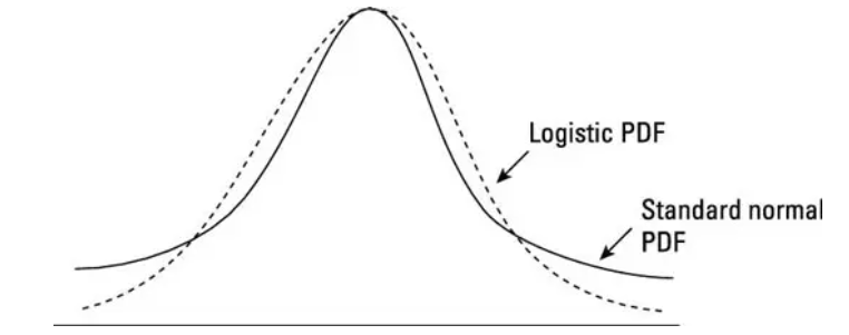
• When we assume $\epsilon$ is follow a normal distribution, this is a probit model (No closed solution)
  • Utility of the variables is considered as a latent variable
• When we assume logistic distribution, this is a logit model
• When we assume gumble distribution, a binomial logit model can be obtained, with the advantages of provbit and logit model